Subdivision scheme ?
Subdivision scheme is the name given to the
parameterization of an iterative process of subdivision.
This subdivision process is usually applied to structured geometric objects : polylines,
polyhedra, polytopes,
meshes.
Each iteration of subdivision breaks a patch of this structure into N new patches.
A patch is defined by a single element of the structure (single segment of a polyline, single polygon of a polyhedron)
and the set of points from the structure "around" this element which play a role in the subdivision of this particular element.
Points of the structure usually have a local influence in the subdivision process. That is, each point of the structure belongs
to the few patches directly adjacent to it and therefore plays a role in the subdivision of the few single geometric elements directly adjacent to it.
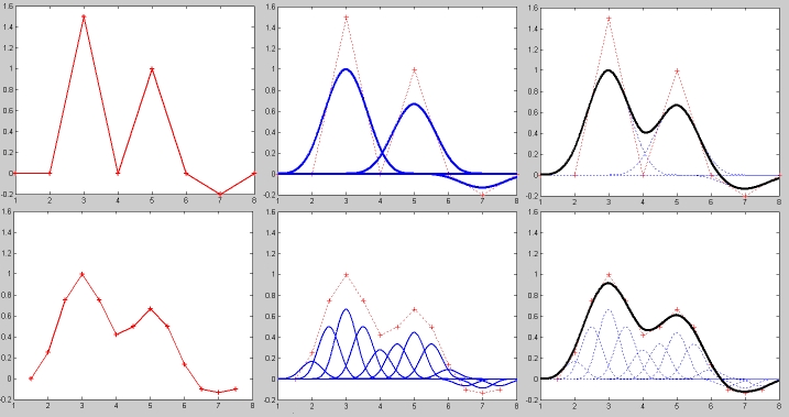
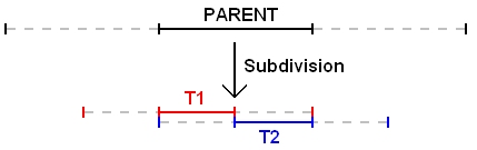
The following figure illustrates a particular subdivision scheme applied to a polyline (upper left). In this particular example a patch is defined by a segment of the polyline
and the 2 points of the polyline directly adjacent to it (so 4 points in total, as colored in red in the upper right figure).
One patch gives, after 1 subdivition iteration, 2 new patches each defined by 4 points (green and blue patches in lower right figure).
These new patches share 3 common points (in cyan), making their segments adjacent.
One iteration of subdivision applied to the whole black polyline returns the blue polyline (bottom left).
The parameters defining the way new patches are created are :
from patch [D,E,F,G], the first blue patch [de,def,eg,efg] is created with the points :
de = (D+E)/2, point de is in the middle of [D,E]
def = (1.D/6 + 4.E/6 + 1.F/6), the position of point def is a linear combination of the positions of the points D,E and F.
ef = (E+F)/2, point ef is in the middle of [E,F]
efg = (1.E/6 + 4.F/6 + 1.G/6), the position of point efg is a linear combination of the positions of the points E,F and G.
You should get the picture for the remaining point of green patch [def,eg,efg,fg].
These subdivision coefficient can be gathered in the stochastic matrices (matrix of which the sum of elements on any column is 1) :
The fact that the two created patches share 3 common points implies that the two matrices share 3 common columns.
The columns of these matrices are the positions of a new patch's points in the barycentric coordinate system of it's parent patch.
These matrices are built in such a way that :
and
The columns of the leftmost matrix in these expressions are the coordinates in our representation space (2D or 3D) of the new patch points,
which are obtained by multiplying the previously defined transform matrices (T1 and T2) with a projection matrix.
The projection matrix's columns are the coordinates in the representation space of the points of the parent patch.
It is a projection matrix from a barycentric space associated to the forementioned barycentric coordinate system to the representation space.
It is very useful to define a subdivision schemes using these barycentric stochastic matrices, as the recursive subdivision of a patch will
come to the building of a transformation tree by performing simple matrix multiplications (as was explained in the introduction page),
and projecting the result in the representation space by another simple matrix multiplication.
The attractor defined in a barycentric space is still invarient relatively to the root object of the tree. Whatever root object we take as primitive
for applying our transforms, the attractor will remain constant in the barycentric space. However, the projection matrix is dependant on the root object control points.
Therefore the attractor's image in the representation space is dependant on the root object's control points. As their names indicate,
control points locally control the image of the attractor in the representation space.
The crucial difference between the IFS presented in the introduction page and the subdivision scheme presented on this page is
the nature of the space in which transforms are defined.
Transforms were, in common IFS, defined in an homogenous space (similar to what we called representation
space on the current page), roughly by a combination of translation, rotation and scaling matrices.
Transforms, in subdivision schemes are represented by higher dimension matrices (as large a dimension as we want) and represent
the coefficient of a linear combination of existing point coordinates.
Commonly used subdivision schemes
Spline curves
The curve subdivision scheme presented above is very widely used in computer graphics. The curve it generates are cubic splines.
The limit by subdivision of a polyline by this scheme is a curve which is equivalent to a curve defined by piecewise cubic polynomes, and which is globally C-2
(continuous and continuous first and second derivatives).
Indeed the curve toward which the subdivided polyline will converge, the IFS attractor, is exactly the curve :
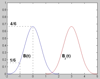
Where the Pi are the points of the original polyline, also called control points of the spline curve, and the Bi are B-Spline functions :
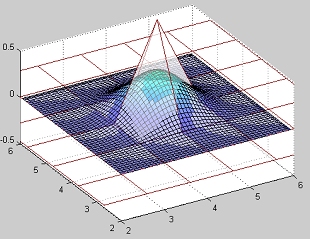
Bspline functions look like this :
A subdivision on the control points polyline creates a new polyline. Each of these polylines (the original, represented in red on the top line of the following figure
and its subdivision on the bottom line) control the same limit spline curve (or IFS attractor, the black polynomial curve).
The change in Bspline functions assossiated to these control points (blue curves in the previous figure) is expressed by what is known as the B-Spline two scale relation :
Catmull Clark surface subdivision scheme
The Catmull-Clark subdivision scheme is to surfaces what the Spline subdivision scheme is to curves. Instead of a polyline, a 2 dimentional regular mesh is subdivided.
The subdivision attractor is also a piecewise cubic polynomial surface, globally C-2. Similarily to the curves,
this Surface can be defined by the polynomes :
Where the Pij are the control points of the original mesh, and the Bij are the tensor products of B-Spline functions :
Curve patch spline subdivision :
Surface patch Catmull-Clark subdivision :
Higher on this page we defined the spline curve subdivion with 2 barycentric matrices : T1 and T2. These matrices expressed the way in which
two new curve patches were created from the points of a parent patch.
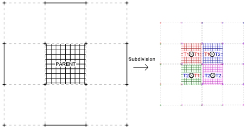
The Catmull-Clark surface subdivision scheme can be defined with 4 matrices.describing the way in which 4 new surface patches are created
from the points of a parent patch.
These matrices are obtained by making the Kronecker products of T1 and T2, their size is therefore 16x16. Surface patches have 16 control points.
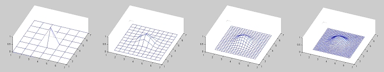
The following strip shows successive subdivisions of a mesh.
The first control mesh and the polynomial surface attractor :
Check out the galleries of IFS structures I created.